We all know that “correlation does not imply causation.” Correlation means X and Y change together, while causation means X makes Y happen. But - as there's a grain of truth in every joke -
seemingly unrelated factors could always be related on some level.
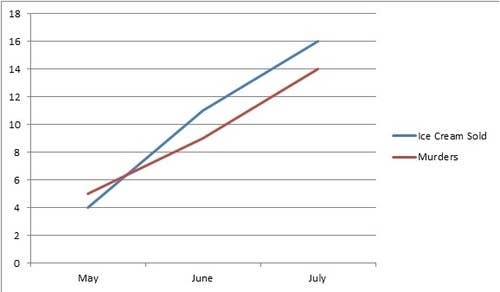
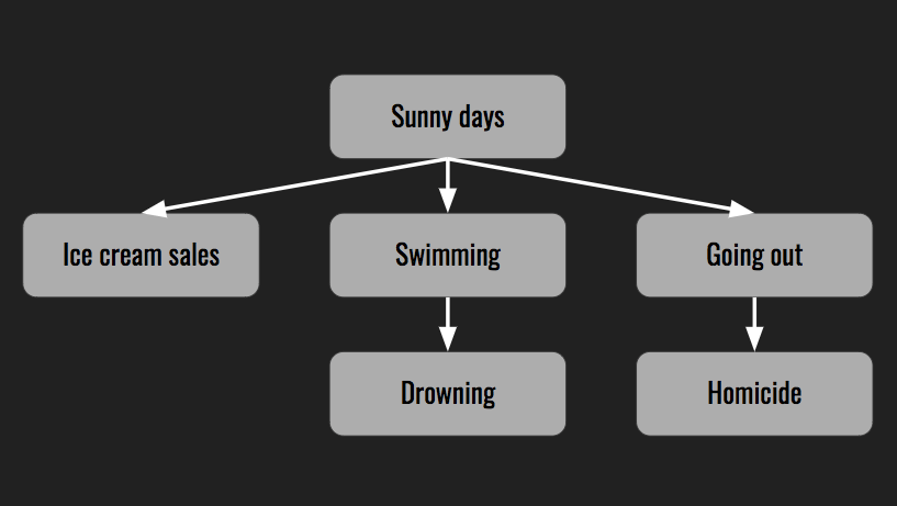
In the case of ice cream sales correlated with drowning death or homicides, the connection is the weather. While soup sales increase during the cold winter months, ice cream sales go up when the temperatures rise. On a nice sunny day more people go for a swim or enjoy the outdoors where there is a wider selection of victims for predators. The most important factor contributing to summer fires is also heat.
The heat wave is an example of a hidden or unseen variable, also known as a confounding variable.
A clinical study might lack control variables - such as the use of placebo. Besides, all possible error sources can't be controlled. But we could reduce the amount of error if we identify all of the possible confounding variables, by a clear understanding of their implications.
How to identify a confounder? By checking if potential confounding factors are associated with both outcome and exposure variables then comparing associations before and after adjusting for it.
Here is an example. Let's assume we studied 100 MEBO patients that experience symptoms after stress and other triggers and 100 patients in remission tolerant to MEBO triggers. 48 participants experienced stress (30 active state, 18 remission) and 152 participants were exposed to low-to-moderate amount of alcohol (82 out of them were in remission). The unadjusted odds ratio (OR) of experiencing symptoms after stress was 1.95 which means that likelihood for flareups was almost twice higher after stress compared to consumption of alcohol)
Unadjusted odds ratio=30×8270×18=1.95
Now we need to find out whether a specific factor, say Bacteria-X, is related to response to stress and/or alcohol. By looking at Table 2, we see that 50% of the patients with flareups and 20% of the patients in remission have detectable levels of this bacteria in their gut.
Odds ratio is a relative risk, a measure of association between an exposure and an outcome. The odds ratio is calculated using the number of case-patients who did or did not have exposure to a (confounding) factor and the number of controls who did or did not have the exposure. The odds ratio tells us how much higher the odds of exposure are among case-patients than among controls.
Suppose 200 persons attended a buffet dinner and 55 attendees became ill after it. We asked everyone to describe what they ate (this is called a case-control study since we compared those with outcome of interest with those who did not have the outcome). 53 of 54 case-patients and 33 of 40 controls mentioned lettuce in their report. The odds of getting sick from lettuce were O1 = 53/33 and the odds of getting sick without eating lettuce was O2 = 1/7, hence the odds ratio for lettuce was about 11.2 (O1/O2)
a = number of persons exposed and with disease 53
b = number of persons exposed but without disease 33
c = number of persons unexposed but with disease 1
d = number of persons unexposed and without disease 7
a+c = total number of persons with disease (case-patients) 54
b+d = total number of persons without disease (controls) 40
a/b divided by c/d = a*d/b*c 53*7/33 = 11.2
Here are real life scenarios from our microbiome study:
Age: a truly confounding variable?
Gender: a truly confounding variable?
REFERENCES
Jager KJ, Zoccali C, Macleod A, Dekker FW. Confounding: what it is and how to deal with it. Kidney international. 2008 Feb 1;73(3):256-60.
Rasmussen SH, Ludeke S, Hjelmborg JV. A major limitation of the direction of causation model: Non-shared environmental confounding. Twin Research and Human Genetics. 2019 Feb;22(1):14-26.
Jing S. A Study on Causal Discovery Considering Confounders.
seemingly unrelated factors could always be related on some level.
 |  |
|---|
In the case of ice cream sales correlated with drowning death or homicides, the connection is the weather. While soup sales increase during the cold winter months, ice cream sales go up when the temperatures rise. On a nice sunny day more people go for a swim or enjoy the outdoors where there is a wider selection of victims for predators. The most important factor contributing to summer fires is also heat.
The heat wave is an example of a hidden or unseen variable, also known as a confounding variable.
 |  |
|---|
How to identify a confounder? By checking if potential confounding factors are associated with both outcome and exposure variables then comparing associations before and after adjusting for it.
Here is an example. Let's assume we studied 100 MEBO patients that experience symptoms after stress and other triggers and 100 patients in remission tolerant to MEBO triggers. 48 participants experienced stress (30 active state, 18 remission) and 152 participants were exposed to low-to-moderate amount of alcohol (82 out of them were in remission). The unadjusted odds ratio (OR) of experiencing symptoms after stress was 1.95 which means that likelihood for flareups was almost twice higher after stress compared to consumption of alcohol)
Table 1
Number of flareups after triggers
| Trigger | MEBO symptoms flareup, no. (%) | ||
|---|---|---|---|
| Flareup | No flareup | Total | |
| Stress | 30 (63) | 18 (37) | 48 |
| Alcohol | 70 (46) | 82 (54) | 152 |
| Total | 100 | 100 | 200 |
Now we need to find out whether a specific factor, say Bacteria-X, is related to response to stress and/or alcohol. By looking at Table 2, we see that 50% of the patients with flareups and 20% of the patients in remission have detectable levels of this bacteria in their gut.
Table 2
Distribution of wound infection cases and controls by Bacteria-X status
| Have Bacteria X | Experiencing flareups | |
|---|---|---|
| Yes | No | |
| No | 50 | 80 |
| Yes | 50 | 20 |
| Total | 100 | 100 |
It seems that, with a ratio of 2.5, Bacteria-X is related to flaareups in response to stress or alcohol. Now we need to understand if this bacteria is acting up in stress vs alcohol conditions. Table 3 shows the relation between Bacteria-X and type of trigger for 200 patients. Of 70 patients with Bacteria-X, 35 (50%) were exposed to high stress and of 130 patients that don't have bacteria-X, 13 (10%) experienced high stress. Thus, with a ratio of 5.0, we clearly observe that patients with bacteria-X were more likely than patients without bacteria-X to experience stress. At this point, it seems that Bacteria-X is related to both stress and alcohol triggers.
Table 3
Relation between type of MEBO trigger and presence of Bacteria-X
| Bacteria-X present | Total | Flareups, no. (%) | |
|---|---|---|---|
| Stress | Alcohol | ||
| No | 130 | 13 (10) | 117 (90) |
| Yes | 70 | 35 (50) | 35 (50) |
Second, we need to calculate the adjusted OR and compare it with the unadjusted OR. We first stratify study population to patients with and without bacteria X. Within each stratum, a contingency (2 × 2) table is created and the OR is calculated (Table 4). When we calculate the OR separately for patients with and without bacteria-X, we find that the OR is 1 in each stratum, indicating the lack of association between flareup and type of stress. We could conclude that the unadjusted OR of 1.95 in Table 1 was owing to the unbalanced distribution of those with bacteria-X in their gut microbiome between cases and controls. Thus, in this example, bacteria-X was a confounder, and the association between stress and MEBO symptoms flareup was spurious.
Table 4
Calculation of odds ratio after stratifying by presence of bacteria X
| Bacteria-X; stress | MEBO flareup, no. (%) | Total | Adjusted odds ratio | |
|---|---|---|---|---|
| Yes | No | |||
| No | ||||
| High | 5 (38) | 8 (62) | 13 | |
| Low | 45 (38) | 72 (62) | 117 | |
| Total | 50 | 80 | 130 | |
| Yes | ||||
| High | 25 (71) | 10 (29) | 35 | |
| Low | 25 (71) | 10 (29) | 35 | |
| Total | 50 | 20 | 70 | |
Confounding can be dealt with at the stage of study design (before collecting the data) or at the stage of data analysis (after collecting the data). The commonly used methods to control for confounding factors and improve internal validity are randomization, restriction, matching, stratification, multi-variable regression analysis and propensity score analysis
Notes about odds ratio
Odds ratio is a relative risk, a measure of association between an exposure and an outcome. The odds ratio is calculated using the number of case-patients who did or did not have exposure to a (confounding) factor and the number of controls who did or did not have the exposure. The odds ratio tells us how much higher the odds of exposure are among case-patients than among controls.
Suppose 200 persons attended a buffet dinner and 55 attendees became ill after it. We asked everyone to describe what they ate (this is called a case-control study since we compared those with outcome of interest with those who did not have the outcome). 53 of 54 case-patients and 33 of 40 controls mentioned lettuce in their report. The odds of getting sick from lettuce were O1 = 53/33 and the odds of getting sick without eating lettuce was O2 = 1/7, hence the odds ratio for lettuce was about 11.2 (O1/O2)
a = number of persons exposed and with disease 53
b = number of persons exposed but without disease 33
c = number of persons unexposed but with disease 1
d = number of persons unexposed and without disease 7
a+c = total number of persons with disease (case-patients) 54
b+d = total number of persons without disease (controls) 40
a/b divided by c/d = a*d/b*c 53*7/33 = 11.2
Here are real life scenarios from our microbiome study:
REFERENCES
Jager KJ, Zoccali C, Macleod A, Dekker FW. Confounding: what it is and how to deal with it. Kidney international. 2008 Feb 1;73(3):256-60.
Rasmussen SH, Ludeke S, Hjelmborg JV. A major limitation of the direction of causation model: Non-shared environmental confounding. Twin Research and Human Genetics. 2019 Feb;22(1):14-26.
Jing S. A Study on Causal Discovery Considering Confounders.